Data science can be intimidating. The truth about the field is that truly every day is a school day and we are learning and improving all the time. Today, I wanted to talk about one of our favourite methods in our ever-expanding analytics toolkit – the rolling join.
As data scientists we regularly join different data sources to get required information. Just some examples could be different radar sources, flight plan data, wind measurements and aircraft parameters. I would consider joins as one of the most powerful data wrangling tools out there.
Inner Joins
To understand what rolling joins are and how they work, it’s important to know what we mean by a “join”. The simplest and most common type of join is known as an “inner” join. Given two tables and a set of joining columns as inputs, the output is a single table, with the joining columns as well as all other columns from both tables. Records only exist in this new table where the joining columns are equal in both tables, hence the term “join”.
The intuition behind a join of two tables can be confusing. I find the best way of thinking about them is to first imagine every record of one table alongside every record of the other side by side. From here, given a set of joining columns, we can remove all combined records that don’t have matching sets of values of these columns.
In Figure 1 below, we look at a inner join of aircraft observations (Table 1) and aircraft wake turbulence category (WTC) values (Table 2). These are joined on the aircraft type column. Matching columns are highlighted in green, and those not matching in red.
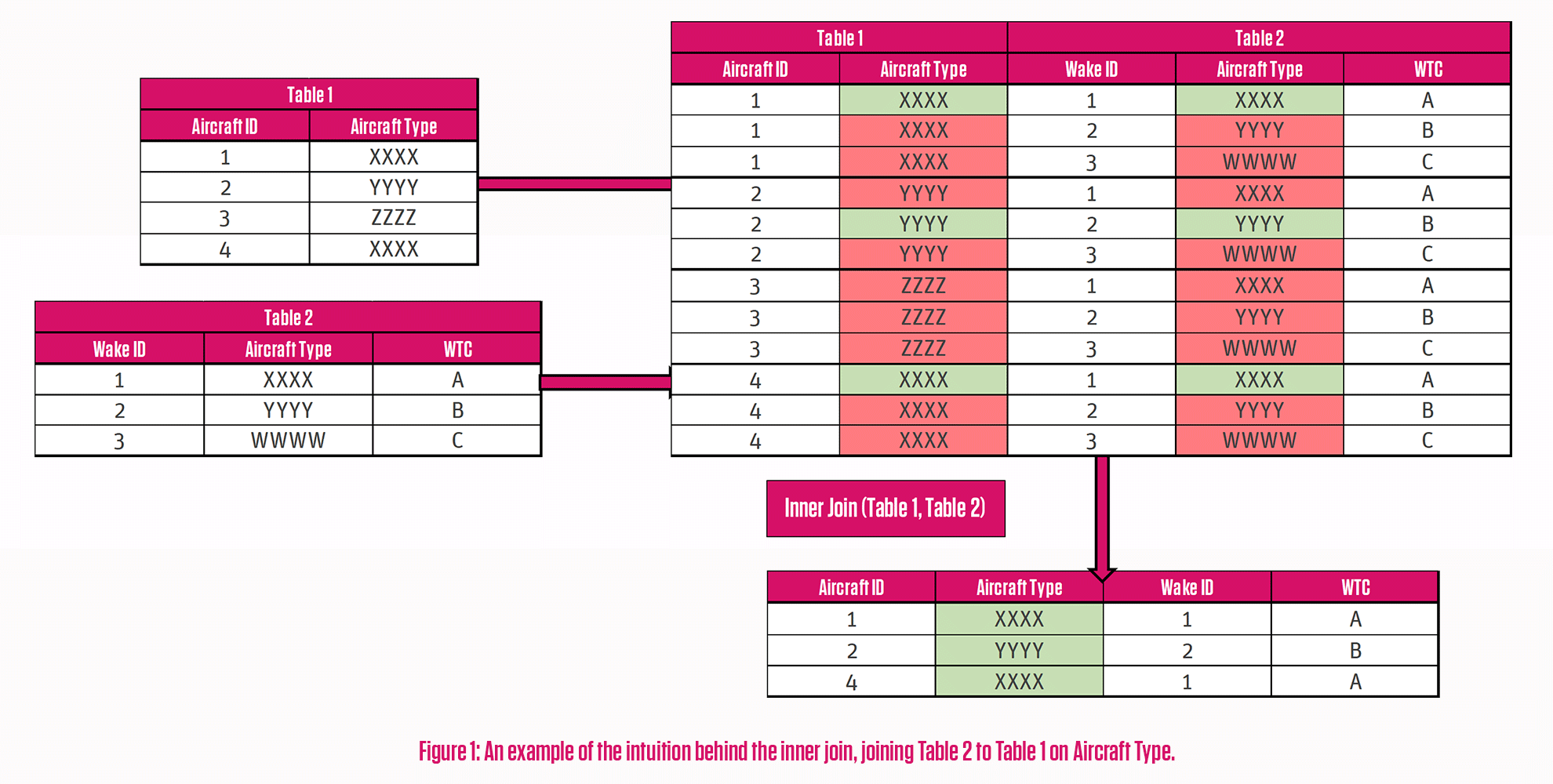
We can see that out of the four aircraft observations, only three remain in the output table. It seems we don’t have a WTC value for the ZZZZ aircraft type!
Extensions to the Natural Join
What if we wanted to retain a record even if there are no matching joining columns?
There exist several “extensions” of the inner join, known as outer joins, which maintain records from one or both tables that don’t provide a match on the joining columns, padding out any columns of the table not containing the joining column values. Left and right outer joins maintain records from the left and right tables respectively, whereas a “full” outer join will maintain records from both, meaning all combinations of joining columns across both tables will remain.
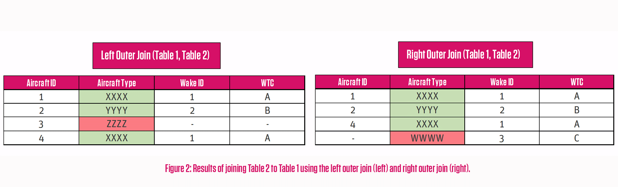
Figure 2 shows the output of a left outer join and a right outer join of Table 1 and Table 2 from Figure 1. In the former, the aircraft observation with ZZZZ is retained, alongside the other column values from Table 1, and for the latter, while this record is removed, the record with the WWWW aircraft type is retained from Table 2.
In practice, I find the left outer join to be the most useful. When joining multiple different datasets together, it is often convenient to maintain the records of the original; but the choice really does depend on the situation.
Rolling Joins
There is one common use case that inner joins and their extensions do not cater for. Imagine a situation where you do not necessarily want columns to just match identically. With all forms of natural joins, you require an exact match between two sets of columns – and this will often leave you with no matches. This occurs frequently in real world data. For example, joining two datasets based on the time of their records. Sometimes, you can’t guarantee observations have been made at the exact same time and you just want to find the nearest record, be that in the past, the future or either direction.
Enter the rolling join, a tool to join datasets based on any number of “fixed” columns (with the same principle as the natural join mechanism and its extensions) and a single, numerical “rolling” column. We can choose how we want this value to “roll”: forwards, backwards, or whatever direction that has the closest match.
What about a case where you don’t want to match observations that are too far away from each other? Rolling joins can handle that too. Simply set a maximum “roll” value along with your direction and you’ll only get a match if there is an observation that falls within that range. You certainly wouldn’t want a wind measurement several hours away from where you’re trying to look!
Rolling joins can be thought of in a similar way to standard joins. Intuitively we can think of all record combinations between the two tables, but as well as finding matches in fixed joining columns, we can look at the differences in the rolling column, and choose records based on these. Figure 3 shows three different rolling join examples with aircraft arrival times (Table 3) and wind measurements (Table 4) based on time: a simple nearest match, a nearest match where the value in Table 3 is below Table 4, and a nearest match within 60 seconds in either direction.
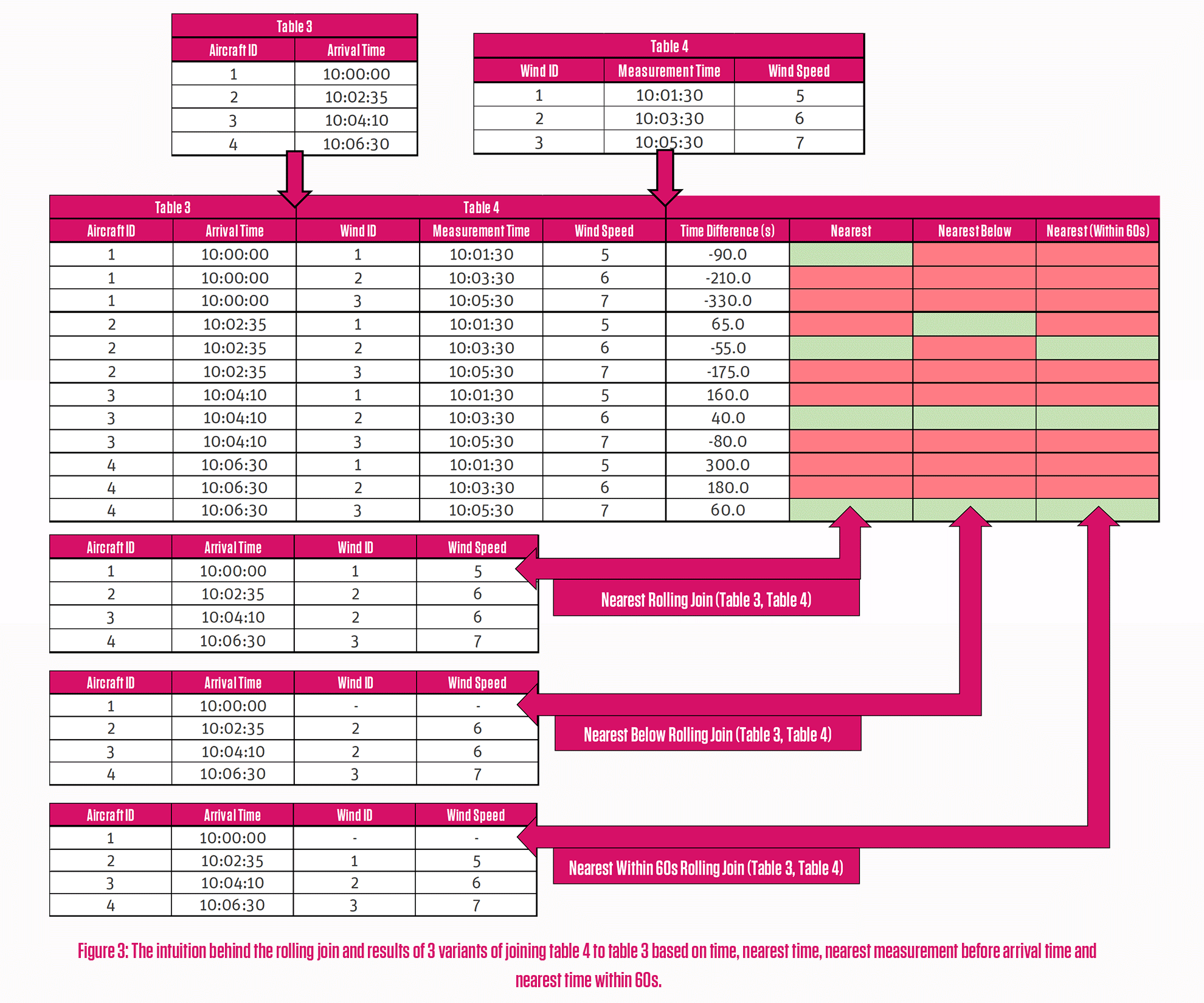
We can see for the second example the first record can’t match to a measurement time as its arrival time is before all the measurements. In the third example, the first record can’t match because there are no measurements within 60 seconds either side of the arrival time. You can start to see how this tool can become useful for a data scientist!
Making use of Rolling Joins
We use the R language for analytics at Think for its plotting capabilities, dashboarding and its data friendly set of tools. One available package in R (data.table) has in built functionality for these types of rolling joins. Where it is possible to replicate this behaviour with a loop, the data.table package has functions optimised for speed, meaning what would take minutes (or even hours!) with a loop will take seconds, if not milliseconds with a rolling join!
One frustrating thing about the use of these rolling joins in R… their syntax can feel quite counter-intuitive. It’s easy to forget what the output data format is going to look like and what columns are going to be removed. We tend to use dplyr as the package of choice for data wrangling because of its easy-to-read functions and syntax. Unfortunately, as far as I’m aware, dplyr, or any other readily available package do not support rolling joins.
To get around this, I decided to create a dplyr style wrapper function to make an easy to read and intuitive way to perform a rolling join. Choose your tables, choose your joining columns, choose the direction and maximum allowed roll value and your second table will join onto the end at the first at the nearest value of the final column in a direction you specify; all in one easy to read code line. I decided to make this in the style of the left outer join, so records from the first table are always retained, and now we use it all the time! It’s as easy as this:
rolling_join(table1, table2, table1cols, table2cols, roll)
Where table2 is to be joined to table1, table1cols and table2cols are vectors of the columns to be joined on, and roll, if used, provides the rolling direction and maximum difference between the rolling columns.
At Think, we’re always looking at new and smarter ways to manipulate our data before using it to get actionable insights for all kinds of analytics projects. Also, like all other human beings, we’re always looking to make things easier for ourselves and those around us. With our operational knowledge, our ever-growing technical expertise and skillset, and our real passion for data, software, and analytics – don’t be afraid to get in touch to see what Think can do for your analytical projects.

Author: George Clark, ATM Consultant
Recent Comments